THE MAIN CONCEPTS AND BUZZWORDS

Most of these terms are introduced early on, within Course 1, Modules 1 – 3.

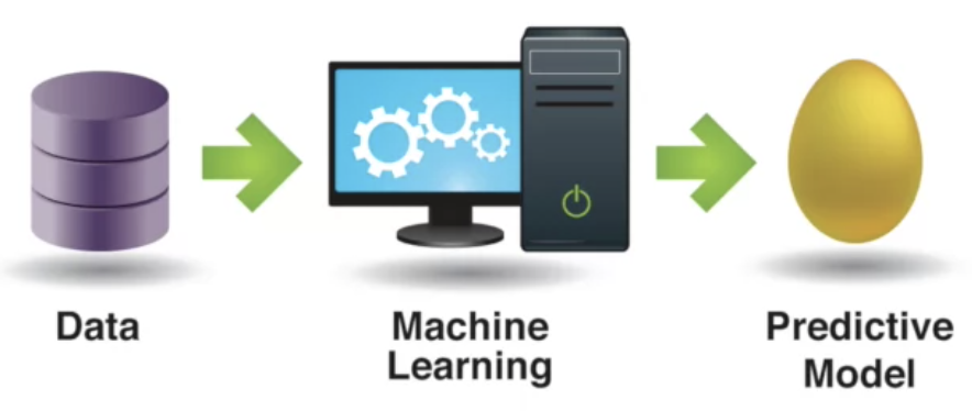
Machine learning: Technology that learns from experience (data) to predict the outcome or behavior of each customer, patient, package delivery, business, vehicle, image, piece of equipment, or other individual unit—in order to drive better operational decisions. ML generates a predictive model whose job is to calculate a predictive score (probability) for each individual.

The ML process is guided by training data, so we say the machine “learns from data” to improve at the task. Specifically, it generates a predictive model from data; the model is the thing that’s “learned”. For business applications of machine learning, the data from which it learns usually consists of a list of prior or known cases (i.e., labeled data). This list of cases amounts to an encoding of “experience”, so the computer “learns from experience”.

Predictive analytics: The use of machine learning for various commercial, industrial, and government applications. All applications of predictive analytics are applications of machine learning, and so the two terms are used somewhat interchangeably, depending on context. However, the reverse is not true: If you use machine learning to, for example, calculate the next best move playing checkers, or to solve certain engineering or signal processing problems, such as calculating the chances a high resolution photo has a traffic light within it, those uses of machine learning are rarely referred to as predictive analytics.

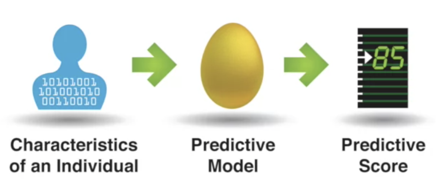
Predictive model: A mechanism that predicts a behavior or outcome for an individual, such as click, buy, lie, or die. It takes characteristics of the individual as input (independent variables) and provides a predictive score as output, usually in the form of a probability. The higher the score, the more likely it is that the individual will exhibit the predicted behavior. Since it is generated by machine learning, we say that a predictive model is the thing that’s “learned”. Because of this, machine learning is also known as predictive modeling.

η Individual: Within the definitions of predictive analytics and predictive model, individual is an intentionally broad term that can refer not only to individual people – such as customers, employees, voters, and healthcare patients – but also to other organizational elements, such as corporate clients, products, vehicles, buildings, manholes, transactions, social media posts, and much more. Whatever the domain, predictive analytics renders predictions over scalable numbers of individuals. That is, it operates at a lower level of granularity. This is what differentiates predictive analytics from forecasting.

Training data: The data from which predictive modeling learns – that is, the data that machine learning software takes as input. It consists of a list (set) of [training] examples, aka training cases. For many business applications of machine learning, it is in the form of one row per example, each example corresponding to one individual

Labeled data: Training data for which the correct answer is already known for each example, that is, for which the behavior or outcome being predicted is already labeled. This provides examples from which to learn, such as a list of customers, each one labeled as to whether or not they made a purchase. In some cases, labeling requires a manual effort, e.g., for determining whether an object such as a stop sign appears within a photograph or whether a certain healthcare condition is indicated within a medical image.

Supervised machine learning: Machine learning that is guided by labeled data. The labels guide or “supervise” the learning process and also serve as the basis with which to evaluate a predictive model. Supervised machine learning is the most common form of machine learning and is the focus of this entire three-course series, so we will generally refer to it simply as machine learning.

Unsupervised machine learning: Methods that attempt to derive insights from unlabeled data. One common method is clustering, which groups examples together by some measure of similarity, trying to form groups that are as “cohesive” as possible. Since there are no correct answers – no labels – with which to assess the resulting groups, it’s generally a subjective choice as to how best to evaluate how good the results of learning are. This three-course series does not cover unsupervised learning (other than giving this definition and as a small part of a one-video case study on fraud detection within Course 3).

Forecasting: Methods that make aggregate predictions on a macroscopic level that apply across individuals. For example: How will the economy fare? Which presidential candidate will win more votes in Ohio? Forecasting estimates the overall total number of ice cream cones that will be purchased next month in Nebraska, while predictive analytics tells you which individual Nebraskans are most likely to be seen with cone in hand.

Data science / big data / analytics / data mining: Beyond “the clever use of data”, these subjective umbrella terms do not have agreed definitions. However, their various, competing definitions do generally include machine learning as a subtopic, as well as other forms of data analysis such as data visualization or, in some cases, just basic reporting. These terms do allude to a vital cultural movement led by thoughtful data wonks and other smart people doing creative things to make value of data. However, they don’t necessarily refer to any particular technology, method, or value proposition.

Artificial intelligence: See this glossary’s section “Artificial intelligence: a problematic buzzword”.

---

 

MACHINE LEARNING APPLICATIONS

Application areas are introduced in Course 1, Module 1 and then revisited in greater depth in Course 2, Module 1.

Machine learning application: A value proposition determined by two elements: 1) What’s predicted: the behavior or outcome to predict with a model for each individual, such as whether they’ll click, buy, lie, or die. And 2) What’s done about it: the operational decision to be driven for each individual by each corresponding prediction; that is, the action taken by the organization in response to or informed by each predictive model output score, such as whether to contact, whether to approve for a credit card, or whether to investigate for fraud.

Deployment: The automation or support of operational decisions that is driven by the probabilistic scores output by a predictive model – that is, the actual launch of the model. This requires the scores to be integrated into operations. For example, target a retention campaign to the top 5% of customers most likely to purchase if contacted. Also known as operationalization, integration, implementation, or “putting a model into production.”

Decision automation: The deployment of a predictive model to drive a series of operational decisions automatically.

Decision support: The deployment of a predictive model to inform operational decisions made by a person. In their decision-making process, the person informally integrates or considers the model’s predictive scores in whatever ad hoc manner they see fit. Also known as human-in-the-loop.

Offline deployment: Scoring a batch job for which speed is not a great concern. For example, when selecting which customer to include for a direct marketing campaign, the computer can take more time, relatively speaking. Milliseconds are usually not a concern.

Real-time deployment: Scoring as quickly as possible to inform an operational decision taking place in real time. For example, deciding which ad to show a customer at the moment a web page is loading means that the model must very quickly receive the customer’s independent variables as input and do its calculations so that the predictive score is then almost immediately available to the operational system.

η The Prediction Effect: A little prediction goes a long way. Predicting better than guessing is very often more than sufficient to render mass scale operations more effective.

η The Data Effect: Data is always predictive. For all intents and purposes, virtually any given data set will reveal predictive insights. Leading UK consultant Tom Khabaza put it this way: “Projects never fail due to lack of patterns.” That is, other pitfalls may derail a machine learning project, but that generally won’t happen because of a lack of value in the data.

Response modeling: For marketing, predictively modeling whether a customer will purchase if contacted in order to decide whether to include them for contact. Also known as propensity modeling.

Churn modeling: For marketing, predictively modeling whether a customer will leave (i.e., defect, cancel, attrite, or leave) in order to decide whether to extend a retention offer.

Workforce churn modeling: Predictively modeling whether an employee will leave (e.g., quit or be terminated) in order to to take measures to retain them or to plan accordingly. Workforce analytics is covered in the Course 2, Module 3 video “Five colorful examples of behavioral data for workforce analytics”.

Credit scoring: For financial services, predictively modeling whether an individual debtor will default or become delinquent on a loan in order to decide whether to approve their application for credit, or to inform what APR and credit limit to offer or approve.

Insurance pricing and selection: Predictively modeling whether an individual will file high claims in order to decide whether to approve their application for insurance coverage (selection) or decide how to price their insurance policy (pricing).

Fraud detection: Predictively modeling whether a transaction or application (e.g., for credit, benefits, or a tax refund) is fraudulent in order to decide whether to have a human auditor screen it.

Product recommendations: Predictively modeling what next product the customer will buy or what media items such as video or music selections that customer would rate highly after consuming it, in order to decide which to recommend.

Ad targeting: Predictively modeling whether the customer will click on – or otherwise respond to – an online advertisement in order to decide which ad to display.

Non-profit fundraising: Predictively modeling whether a prospect will donate if contacted in order to decide whether to include them for contact. This is the same value proposition as with response modeling for marketing, except that “order fulfillment” is simpler: Rather than sending each responder a product, you only need to send a “thank you” note.

Algorithmic trading: Predictively modeling whether an asset’s value will go up or down in order to drive trading decisions.

Predictive policing: Predictively modeling whether a suspect or convict will be arrested or convicted for a crime in order to inform investigation, bail, sentencing, or parole decisions. One typical modeling goal is to predict recidivism, that is, whether the individual will be re-arrested or re-convicted upon release from serving a jail sentence. Predictive policing is covered in the Course 2, Module 4 video “Predictive policing in law enforcement and national security”.

η Automatic suspect discovery (ADS): In law enforcement, the identification of previously unknown potential suspects by applying predictive analytics to flag and rank individuals according to their likelihood to be worthy of investigation, either because of their direct involvement in, or relationship to, criminal activities. A note on automation: ADS flags new persons of interest who may then be elevated to suspect by an ensuing investigation. By the formal law enforcement definition of the word, an individual would not be classified as a suspect by a computer, only by a law enforcement officer. ADS is not covered in this course – click here for more information.

Fault detection: For manufacturing, predictively modeling whether an item or product is defective – based on inputs from factory sensors – in order to decide whether to have it inspected by a human expert.

Predictive maintenance: Predictively modeling whether a vehicle or piece of equipment will fail or break down in order to decide whether to perform routine maintenance or otherwise inspect the item.

Image classification: Predictively modeling whether an image belongs to a certain category or depicts a certain item or object (aka object recognition) within it in order to automatically flag the image accordingly. Applications of image classification include face recognition and medical image processing.

---

 

THE TRAINING DATA

Training data and its preparation are introduced in Course 1, Module 2 and then covered more extensively in Course 2, Module 3.

Note: See also this glossary’s section “The main concepts and buzzwords” (above) for the definitions of these related terms: training data, labeled data, and individual.

Data preparation: The design and formation of the training data. This normally requires a specialized engineering and database programming effort, which must be heavily informed by business consideration, since the training data defines the functional intent of the predictive model that will be generated from that data.

Predictive goal: The thing that a model predicts, its target of prediction – that is, the outcome or behavior that the model will predict for each individual. For a given individual being predicted by the model, the score output by the model corresponds with the probability of this outcome or behavior. For example, this is a hypothetical predictive goal for churn modeling: “Which current customers with a tenure of at least one year and who have purchased more than $500 to date will cancel within three months and not rejoin for another three months thereafter?” Also known as prediction goal or predictive objective.

Dependent variable: The value, for each example in the training data, which corresponds with the predictive goal. This is what makes the data labeled; for each training example, the dependent variable’s value is that example’s label. Only labeled data has a dependent variable; unlabeled data is by definition data that does not have a dependent variable. The dependent variable is often positioned as the rightmost column of the table of training data, although that is not a strict convention. Also known as output variable.

Independent variable: A factor (i.e., a characteristic or attribute) known about an individual, such as a demographic like age or gender, or a behavioral variable such as the number of prior purchases. A predictive model takes independent variables as input. Also known as feature or input variable.

Binary classifier. A predictive model that predicts a “yes/no” predictive goal, i.e., whether or not an individual will exhibit the outcome or behavior being predicted. When predictively modeling on training data with a dependent variable that has only two possible values, such as “yes” and “no” or “positive” and “negative”, the resulting model is a binary classifier. Binary classifiers suffice, at least as a first-pass approach, for most business applications of machine learning. This three-course series only covers binary classification – it does not cover models that predict more values, such as for predicting “how much spent” or “how many purchased”.

Positive and negative examples. In binary classification, the two possible outcomes or behaviors are usually signified as “positive” and “negative”, but it is somewhat arbitrary which is considered which. In most cases, the positive class is the less frequent class and is also the one that is more valuable to correctly identify, such as emails that are spam, medical images that signify the presence of a disease, or customers who will churn.

Test data: Data that is held aside during the modeling process and used only to evaluate a model after the modeling is complete. The test data has the same variables as the training data, the same set of independent variables and the same dependent variable.

Demographic data: Independent variables that characterize who an individual is. These are inherent characteristics that are either immutable or tend not to change often, such as gender, age, ethnicity, aspects of the postal address, and billing details. Sometimes referred to as profile data.

Behavioral data: Independent variables that summarize what an individual has done or what has happened to that individual. This includes purchase behavior, online behavior, or any other observations of the individual’s actions.

Derived variable: A manually-engineered independent variable inserted into the training data that is intended to provide value to the predictive model (typically, this means inserting a new column). A derived variable builds on other independent variables, extracting information through often simple mathematical operations. Deriving new independent variables is known as feature engineering or feature discovery (never “independent variable derivation” or anything like that, as it turns out).

Feature selection: An automatic or semi-automatic pre-modeling phase that selects a favored subset of independent variables to be used for predictive modeling. After setting aside (filtering out) less valuable or redundant independent variables, the predictive modeling process has fewer independent variables to contend with and can “focus” only on a smaller number of valuable independent variables. This can result in a predictive model that exhibits higher performance.

---

 

THE CORE ALGORITHMS: MACHINE LEARNING METHODS

The general concepts behind machine learning methods (and the basics of decision trees specifically) are introduced in Course , Modules 2 – 3 and then more extensive coverage that dives into each of several algorithms comes in Course 3, Modules 1 – 3.

Algorithm: A well-defined process that solves a problem. Note that this is a general computer science term – it isn’t specific to the field of machine learning. In practice, the word algorithm essentially means any problem-solving method that is defined specifically-enough that you could program a computer to do it. A complete definition of algorithm also spells out other requirements, such as that it must take a finite amount of time rather than running forever, that it must designate a result as its output – a result that is the solution to whatever problem the algorithm is solving – and that it be unambiguous and computable (i.e., doable/executable). However, the shorter definition “a well-defined process that solves a problem” suffices for our purposes here. In the context of machine learning, the term algorithm mostly serves to refer to a modeling method – such as decision trees or logistic regression – in the abstract, i.e., without reference to any specific software tool that implements it.

Predictive modeling method: An algorithm to generate a predictive model. Also known as a machine learning algorithm or a machine learning method. The following modeling methods are covered by the three-course series with greatest detail in Course 3: decision trees, Naive Bayes, linear modeling, perceptrons, logistic regression, neural networks, deep learning, ensemble models, and uplift modeling.

Uplift modeling: Predictive modeling to predict the influence on an individual‘s behavior or outcome that results from choosing one treatment over another. Instead of predicting the future, the behavior, whether there will be a positive outcome – as done by traditional predictive modeling – an uplift model predicts, “How much more likely is this treatment to result in the desired outcome than the alternative treatment?” For marketing, it predicts purchases because of contact rather than in light of contact. Uplift modeling is covered by a sequence of three videos within Course 3, Module 3. Also known as persuasion modeling, net lift modeling, true lift modeling, differential response modeling, impact modeling, incremental impact modeling, incremental lift modeling, net response modeling, and true response modeling.

Induction: The act of generalizing from examples, of leaping from a set of particulars to universals. Predictive modeling is a type of induction.

Deduction: The act of reasoning from the general to the particular, such as when applying known rules. For example, if all men are mortal and Socrates is a man, then deduction tells us Socrates is mortal. The application of a predictive model to score an individual is an act of deduction, while the generation of the model in the first place is an act of induction. Induction ascertains new knowledge and deduction applies that knowledge. Induction almost always presents a greater challenge than deduction. Also known as inference.

Decision boundaries: The boundaries that represent how a predictive model classifies individuals, when viewing the “space of individuals” as positioned on a two- or three-dimensional grid. This is a method to visually depict and help people gain an intuitive understanding of how a predictive model operates, the outward effects of its inner workings, what it mechanically accomplishes (without necessarily understanding how it works mathematically). When individuals are positioned within a higher dimensional space beyond two or three dimensions, that is, by considering more than three independent variables, it is not possible for humans to intuitively visualize. For that reason, this method is limited to only helping when a very small number of independent variables are in use.

AutoML (automated machine learning): Machine learning software capabilities that automate some of the data preparation, feature selection, feature engineering, selection of the modeling algorithm itself, and setting of the parameters for that choice of algorithm. While machine learning algorithms are themselves already automatic (by definition), autoML attempts to automate traditionally manual steps needed to set up and prepare for the use of those algorithms.

---

 

HOW WELL ML WORKS: MEASURING ITS PERFORMANCE

This course series emphasizes lift more than any other model performance metric, introducing it in Course 1, Module 1 and covering it more extensively in Course 2, Module 1. Gains curves, which are closely related to lift, are also emphasized, covered in detail in Course 2, Module 1 and then used throughout Course 3, Modules 1 – 3 (to demonstrate the performance of the various modeling methods covered). Many of the other metrics listed here are covered in the first half of Course 2, Module 4.

Accuracy: The proportion of cases a predictive model predicts correctly, that is, how often the model is correct. Accuracy does not differentiate between how often the model is correct for positive and negative examples. This means that, for example, a model with high accuracy could in fact get none of the positive cases correct, if positive examples are relatively rare.

Lift: A multiplier – how many times more often the positive class occurs within a given segment defined by a predictive model, in comparison with the overall frequency of positive cases. We say that a predictive model achieves a certain lift for a given segment. For example, “This model achieves a lift of three for the top 20%. If marketed to, the 20% of customers predicted as most likely to buy are three times more likely than average to purchase.”

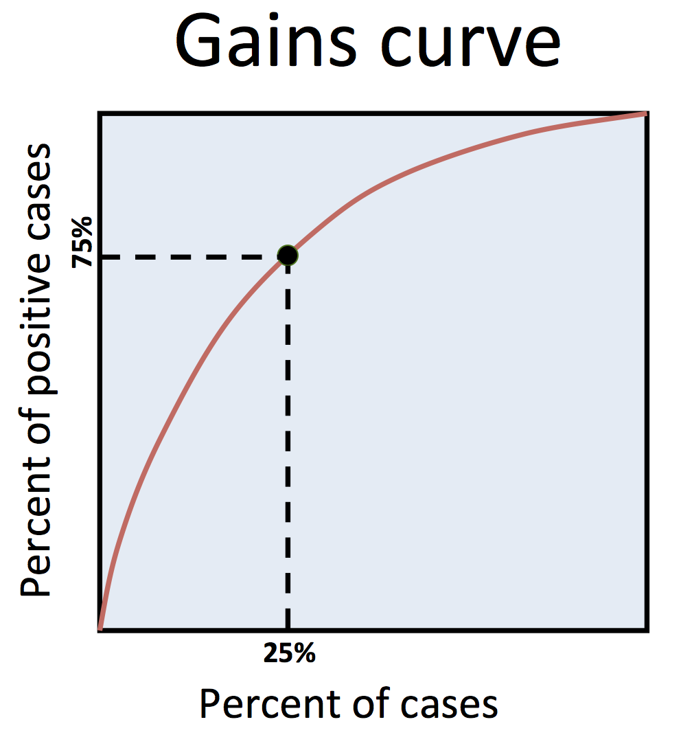
Gains curve: A depiction of predictive model performance with the horizontal axis signifying the proportion of examples considered, as ordered by model score, and the vertical axis signifying the proportion of all positive cases found therein. For example, for marketing, the x-axis represents how many of the ranked individuals are contacted, and the y-axis conveys the percent of all possible buyers found among those contacted. The gains curve corresponds with lift since, at each position on the x-axis, the number of times higher the y-value is in comparison to the x-value equals the lift (equivalently, the number of times higher the curve is in comparison to the horizontally corresponding position on a straight diagonal line that extends from the bottom-left to the top-right equals the lift). Somewhat commonly, gains curves are incorrectly called “lift curves” – however, a lift curve is different. It has lift as its vertical axis, so it starts at the top-left and meanders down-right (lift curves are not covered in this course series).

Profit curve: A depiction of predictive model performance with the same horizontal axis as a gains curve – signifying the proportion of examples considered – and with the vertical axis signifying profit. For example, for direct marketing, the x-axis is how many of the ranked individuals are to be contacted, and the y-axis is the profit that would be attained with that marketing campaign. To draw a profit curve, two business-side variables must be known: the cost per contact and the profit per positive case contacted.

False positive: When a predictive model says “positive” but is wrong. It’s a negative case that’s been wrongly flagged by the model as positive. Also known as false alarm.

False negative: When a predictive model says “negative” but is wrong. It’s a positive case that’s been wrongly flagged by the model as negative.

Misclassification cost: The penalty or price assigned to each false positive or false negative. For example, in direct marketing, if it costs $2 to mail each customer a brochure, that is the false positive cost – if the model incorrectly designates a customer as a positive case, predicting that they will buy if contacted, the marketing campaign will spend the $2, but to no avail. And, if the average profit from each responsive customer is $100, that is the false negative cost – if the model incorrectly designates a customer as a negative case, the marketing campaign will neglect to contact that customer, and will thereby miss the opportunity to earn $100 from them. Misclassification costs form a basis for evaluating models – and, in some cases, for how modeling algorithms generate models, by designating the metric the algorithm is designed to optimize. In that way, costs can serve to define and determine what a machine learning project aims to optimize.

Pairing test: An (often misleading) method to evaluate predictive models that tests how often a model correctly distinguishes between a given pair of individuals, one positive and one negative. For example, if shown two images, one with a cat (meow) and one without a cat (no meow), how often will the model score the positive example more highly and thereby succeed in selecting between the two? This presumes the existence of such pairs, each already known to include one positive case and one negative case – however, the ability to manufacture such test pairs would require that the problem being approached with modeling has already been solved. A model’s performance on the pairing test is mathematically equal to its AUC. The performance on the pairing test is often incorrectly confused or conflated with accuracy.

AUC (Area Under the receiver operating characteristic Curve): A metric that indicates the extent of performance trade-offs available for a given predictive model. The higher the AUC, the better the trade-off options offered by the predictive model. The AUC is mathematically equal to the result you get running the pairing test. The AUC is outside the scope of this three-course series. It is a well-known but controversial metric.

ROC (Receiver Operating Characteristic curve): A curve depicting the true positive rate vs. the false positive rate of a predictive model. The vertical axis, true positive rate, is the same as for a gains curve. Fluency with the ROC is outside the scope of this three-course series. It often visually appears somewhat similar to a gains curve in its shape, but the horizontal axis is the number of negative cases you’ve seen so far, rather than the total number of cases – positive or negative – as in a gains curve.

The following two terms, KPI and strategic objective, are covered in the Course 2, Module 2 video “Strategic objectives and key performance indicators”.

Key performance indicator (KPI): A measure of operational business performance that is key to a business’s strategy. Examples include revenue, sales, return on investment (ROI), marketing response rate, customer attrition rate, market penetration, and average wallet share. Also known as a success metric or a performance measure.

Strategic objective: A KPI target used as a basis for reporting on the business improvements achieved by machine learning. Achieving a strategic objective by incorporating a predictive model is a key selling point for that model. A strategic objective must define a KPI target that:

• Aligns with organizational objectives
• Compels colleagues in order to achieve ML project buy-in
• Is measurable, in order to track ML success
• Is possible to estimate a priori

---

 

THE BUSINESS SIDE: MACHINE LEARNING PROJECT LEADERSHIP

Project leadership is covered in Course 2, Module 2. Note that the five terms defined in this section are less standard than most other terms in this glossary – the concepts are fairly universal, but the nomenclature for these concepts varies widely.

η BizML: The strategic and tactical practice for running an ML project so that it successfully deploys, formulated as a six-step playbook:

1. Value: Establish the deployment goal.

2. Target: Establish the prediction goal.

3. Performance: Establish the evaluation metrics.

4. Fuel: Prepare the data.

5. Algorithm: Train the model.

6. Launch: Deploy the model.

BizML was introduced by the book The AI Playbook: Mastering the Rare Art of Machine Learning Deployment. This kind of business management process is also known as an analytics lifecycle, standard process model, implementation guide, or organizational process.

Project leader: The machine learning team member who keeps the project moving and on track, seeking to overcome process bottlenecks and to ensure that the technical process remains business-relevant, on target to deliver business value. Also known as project manager.

Data engineer: The machine learning team member who prepares the training data. She or he is responsible for sourcing, accessing, querying, and manipulating the data, getting it into its required form and format: one row per training example, each row consisting of various independent variables as well as the dependent variable. This role will often be split across multiple people, since it involves miscellaneous tasks normally suited to DBAs and database programmers, and often involving multiple technologies such as cloud computing and high-bandwidth data pipelines. Team members who perform some of these tasks are sometimes also referred to as data wranglers.

Predictive modeler: The machine learning team member who creates one or more predictive models by using a machine learning algorithm on the training data. This is a technical, hands-on practitioner with experience operating machine learning software.

Operational liaison: The machine learning team member who facilitates the deployment of predictive models, ensuring the model is successfully integrated into existing operations.

---

 

PITFALLS: COMMON ERRORS AND SNAFUS

These pitfalls are covered throughout Course 2 and Course 3. For an overview of the pitfalls that points out specifically where each pitfall is covered within the courses, watch the video “Pitfalls – the seven deadly sins of machine learning”, in Course 3, Module 4.

Overfitting: When a predictive model’s performance on the test data is significantly worse than its performance on the training data used to create it. To put it another way, this is when modeling has discovered patterns in the training data that don’t hold up as strongly in general. This definition is subjective, since “significantly” is not specified exactly. It might overfit just a bit and not really be considered overfitting. And the model might overfit some and yet still be a good enough model. In other cases, a model may completely “flatline” on the test data, in which case, it has overtly overfit. But where the line’s drawn between the two isn’t definitive. Also known as overlearning.

P-hacking: Systematically trying out enough independent variables – or, more generally, testing enough hypotheses – that you increase the risk of stumbling upon a false correlation that, when considered in isolation, appears to hold true, since it passes a test for statistical significance (i.e., shows a low p-value), albeit only by random chance. This leads to drawing a false conclusion, unless the number of variables tried out is taken into account when assessing the integrity of any given discovery/insight. The ultimate example of “torturing data until it confesses”, to p-hack is to try out too many variables/hypotheses, resulting in a high risk of being fooled by randomness. P-hacking is is a variation of overfitting, but rather than with complex models, it happens with very simple, one-variable models. Also known as data dredging, cherry-picking findings, vast search, look-elsewhere effect, significance chasing, multiple comparisons trap, researcher degrees of freedom, the garden of forking paths, data fishing, data butchery, or the curse of dimensionality.

η The accuracy fallacy: When researchers report the high “accuracy” of a predictive model, but then later reveal – oftentimes buried within the details of a technical paper – that they were actually misusing the word “accuracy” to mean another measure of performance related to accuracy but in actuality not nearly as impressive, such as the pairing test or the classification accuracy if half the cases were positive. This is a prevalent way in which machine learning performance is publicly misconstrued and greatly exaggerated, misleading people at large to falsely believe, for example, that machine learning can reliably predict whether you’re gay, whether you’ll develop psychosis, whether you’ll have a heart attack, whether you’re a criminal, and whether your unpublished book will be a bestseller.

Presuming that correlation implies causation: When operating on found data that has no control group, the unwarranted presumption of a causative relationship based only on an ascertained correlation. For example, if we observe that people who eat chocolate are thinner, we cannot jump to the presumption that eating chocolate actually keeps you thinner. It may be that people who are thin eat more chocolate because they weren’t concerned with losing weight in the first place, or any of a number of other plausible explanations. Instead, we must adhere to the well known adage, “Correlation does not imply causation.”

Optimizing for response rate: In marketing applications, conflating campaign response rate with campaign effectiveness. If many individuals who are targeted for contact do subsequently make a purchase, how do you know they wouldn’t have done so anyway, without spending the money to contact them? It may be that you’re targeting those likely to buy in any case – the “sure things” – more than those likely to be influenced by your marketing. The pitfall here is not only in how one evaluates the performance of targeted marketing, it is in whether one models the right thing in the first place. In many cases, a marketing campaign receives a lot more credit than it deserves. The remedy is to employ uplift modeling, which predicts a marketing treatment’s influence on outcome rather than only predicting the outcome.

Data leak: When an independent variable gives away the dependent variable. This is usually done inadvertently, but, informally, is referred to as “cheating”, since it means the model predicts based in part on the very thing it is predicting. This overblows the reported performance as evaluated on the test data, since that performance cannot be matched when going to deployment, since the future will not be encoded within any independent variable (it cannot be, since it is not yet known). For example, if you’re doing churn modeling, but an independent variable includes whether the customer received a marketing campaign contact that had only later been applied to customers who hadn’t cancelled their subscription, then the model will very quickly figure out that this is a helpful way to predict churn.

---

 

ARTIFICIAL INTELLIGENCE: A PROBLEMATIC BUZZWORD

This is an unusual section for a glossary to have, since it focuses on a term for which, in the context of engineering, there can be no satisfactory definition. The author/instructor covers these issues in the Harvard Business Review article “The AI Hype Cycle Is Distracting Companies.” The issues with “artificial intelligence” are also covered in greater detail by the following three consecutive videos within Course 1, Module 4:

• “Why machine learning isn’t becoming superintelligent”
• “Dismantling the logical fallacy that is AI”
• “Why legitimizing AI as a field incurs great cost”

Artificial intelligence (AI): A subjective term with no agreed definition that is intended to inspire technological development, but oversells both current capabilities and the trajectory of today’s technological progress. As an abstract notion, AI can inspire creative thought. However, AI is represented as not just an idea but as an established field. As such, most uses of the term AI tacitly convey misinformation.

THE TWO MAIN PROBLEMS WITH THE TERM AI:

1. “Intelligence” is a subjective idea, not a formally-defined goal pursuable by engineering. Giving the name “artificial intelligence” to a field of engineering conveys, “We’re going to build intelligence.” But such a pursuit cannot succeed because it has set a subjective goal. Because it is a subjective concept, intelligence is not a pursuable objective for engineering. With no objective benchmark by which to evaluate the thing they’re trying to build, pursuers of “AI” cannot keep the construction going in a clearly-defined direction and could never establish “success” if and when it were achieved. However, there are (vain) attempts to resolve this problem by agreeing upon an objective goal. These attempts generally follow one of two approaches, which correspond with the first two definitions of AI listed below.
2. The term AI falsely implies that current technological improvement follows a trajectory towards human-like or human-level capabilities, but the established methods that are referenced as pertinent, such as supervised machine learning, are not designed to do so. One can speculate that other yet-unknown, forthcoming methods could someday emerge and take the lead – indeed, such speculation has been a common pastime since at least 1950. However, establishing a well-defined, pertinent goal for such methods faces the same problem as for existing methods (see the prior paragraph).

THE VARIOUS COMPETING DEFINITIONS OF AI FAIL TO SUFFICE:

 

In its general use, the term AI promulgates The Great AI Myth, falsely suggesting technological development that does not exist. To date, the most prominent, established method to get computers to “program themselves” to accomplish challenging tasks is supervised machine learning, which is intrinsically limited to the pursuit of well-defined tasks by its need for an objective measure of performance and, as a result of that, for many applications, the need for labeled data. Speculating on advancements towards artificial general intelligence is no different now, even after the last several decades of striking innovations, than it was back in 1950, when Alan Turing, the father of computer science, first philosophized about how the word “intelligence” might apply to computers (cf. the Turing Test).

η The Great AI Myth: The belief that technological progress is advancing along a continuum of better and better general intelligence to eventually surpass human intelligence, i.e., achieve superintelligence. As quickly as technology may be advancing, there’s no basis for presuming it is headed towards “human-like” or “human-level” capabilities, since there is no established technology or field of research that is intrinsically designed to do so.

Narrow AI: AI focused on one narrow, well-defined task. Although the AI part of this term defies definition (as discussed in its entry of this glossary, above), in its general usage, the term narrow AI essentially means the same thing as supervised machine learning. However, in most cases, people use the term AI without clarifying whether they mean narrow AI or AGI.

Artificial general intelligence (AGI): AI that extends beyond narrow AI to achieve the capabilities of “real” or “full” AI, i.e., the subjective realm of capabilities people generally intend to allude to when using the term artificial intelligence. Competing definitions include systems that achieve intelligence equal to a human, that achieve superintelligence, or that can undertake all tasks as well as a human. As such, fully defining AGI and legitimizing it as a field faces the same dilemmas as for AI: outright subjectivity and a lack of a clearly-defined goal.

Superintelligence: Intelligence that surpasses human intelligence. Intelligence is a purely subjective notion and, due to The AI Effect, there is no conceivable benchmark for comparing relative degrees of machine intelligence that would not become quickly outdated. For that reason, superintelligence could never be conclusively established.

The AI Effect: An argument that the definition of artificial intelligence is an endlessly moving target, forever out of reach (unachievable), since, once a computer can accomplish any given task thought to require intelligence, the mechanical steps of the computer are fully known and therefore seem (subjectively) “mundane” and no longer seem (subjectively) to require “intelligence” in the full meaning intended by the term AI. That is, once a computer can do it, it seems less “impressive” and loses its “charm”. The late computer science pioneer Larry Tesler suggested that the “intelligence” of AI be paradoxically defined as “whatever machines haven’t done yet.” Given this definition, AI is intrinsically unachievable. Also known as Tesler’s Theorem.

Turing Test: A benchmark for machine intelligence developed by Alan Turing. If a system consistently fools people into believing it’s human, it passes the test – for example, by responding to questions in a chatroom-like setup. This benchmark is a moving target, since humans, who serve as subjects in the experiment, continually become wiser to the trickery used to fool them. When a system passes the Turing Test, humans subsequently figure out a way to defeat it, such as a new line of questioning that reveals which is a human and which is not.

η Quixotic coding: The author/instructor’s preferred term for the “field” known as artificial intelligence. Look, I’m not totally joking – let’s call it that.

Cognitive computing: Another subjectively-defined “field” inspired by human capabilities that is closely related or identical to artificial intelligence and faces the same problems as AI: a lack of a well-defined goal and the overselling of both current capabilities and of the trajectory of today’s technological progress.

---

 

MACHINE LEARNING ETHICS: SOCIAL JUSTICE CONCERNS

Machine learning ethics is covered within Module 4 of each of the three courses.

Protected class: A demographic group designated to be protected from discrimination or bias. Independent variables that impart membership in a protected class include race, religion, national origin, gender, gender identity, sexual orientation, pregnancy, and disability status.

η Discriminatory model: A predictive model that incorporates one or more independent variables that impart membership in a protected class. By taking such a variable as an input, the model’s outputs – and the decisions driven by the model – are based at least in part on membership in a protected class. Exceptions apply when decisions are intended to benefit a protected class, such as for affirmative action, when determining whether one qualifies for a grant given to members of a protected class, or when determining medical treatment by gender.

Machine bias: When a predictive model exhibits disparate false positive rates between protected classes, such as a crime risk model that exhibits a higher false positive rate for black defendants than for white defendants. While the word bias is a relatively broad and subjective criterion in its general usage, this definition applies consistently across this three-course series. Also known as algorithmic bias.

Ground truth. Objective reality that may or may not be captured by data, especially in relation to the dependent variable. For example, if training data used to develop a crime risk model includes arrests or convictions for its dependent variable, there is a lack of ground truth, since arrests or convictions are only a proxy to whether an individual committed a crime (not all crimes are known and prosecuted).

Explainable machine learning: Technical methods to help humans understand how a predictive model works. Also known as explainable AI.

Model transparency: The standard that predictive models be accessible, inspectable, and understandable. In some cases, this is only a matter of authorizing access to models for an auditing process that may include both model inspection and interrogation (experimentation). In other cases, it also requires the use of explainable machine learning, since, once accessed, a more complex model may require special measures in order to decipher it.

The right to explanation: The standard that model transparency be met when a consequential decision is driven or informed by a predictive model. For example, a defendant would be told which independent variables contributed to their crime risk score – for which aspects of his or her background, circumstances, or past behavior the defendant was penalized. This provides the defendant the opportunity to respond accordingly, providing context, explanations, or perspective on these factors.

Predatory micro-targeting: When machine learning‘s increase in efficiency of activities designed to maximize profit leads to the disenfranchisement of consumers. Examples include when financial institutions are empowered to hold individuals in financial debt or when highly targeted advertisements are made increasingly adept at exploiting vulnerable consumers. In general, improving the micro-targeting of marketing and the predictive pricing of insurance and credit can magnify the cycle of poverty for consumers.

The Coded Gaze: If a group of people such as a protected class is underrepresented in the training data used to form a predictive model, the model will, in general, not work as well for members of that group. This results in exclusionary experiences and discriminatory practices. This phenomenon can occur for both facial image processing and speech recognition. Also known as representation bias.

---

 

η Terms marked with this symbol were newly introduced by this course series (or within previous writing by the instructor, Eric Siegel).

ALPHABETICAL INDEX

accuracy
the accuracy fallacy η
AUC (Area Under the receiver operating characteristic Curve)
automatic suspect discovery (ASD) η
ad targeting
algorithm
algorithmic trading
analytics
artificial general intelligence (AGI)
artificial intelligence (AI)
The AI Effect
autoML
behavioral data
big data
bizML
churn modeling
The Coded Gaze
cognitive computing
credit scoring
The Data Effect η
data engineer
data leak
data mining
data preparation
data science
decision automation
decision boundaries
decision support
deduction
demographic data
dependent variable
deployment
derived variable
discriminatory model η
explainable machine learning
false negative
false positive
fault detection
feature selection
forecasting
fraud detection
gains curve
The Great AI Myth η
image classification
independent variable
individual η
induction
insurance pricing and selection
key performance indicator (KPI)
labeled data
lift
machine bias
machine learning
machine learning application
misclassification cost
model transparency
narrow AI
non-profit fundraising
offline deployment
operational liaison
optimizing for response rate
overfitting
p-hacking
pairing test
The Prediction Effect η
predictive analytics
predictive goal
predictive maintenance
predictive model
predictive modeler
predictive modeling method
predictive policing
presuming that correlation implies causation
product recommendations
profit curve
project leader
protected class
quixotic coding η
real-time deployment
response modeling
the right to explanation
ROC (Receiver Operating Characteristic curve)
strategic objective
superintelligence
supervised machine learning
test data
training data
Turing Test
unsupervised machine learning
workforce churn modeling